1 Introduction to Web Data Science
- Articulate what distinguishes web data science from general data science
- Set up a reproducible computing environment with Anaconda, Python, and Jupyter Notebooks
- Make a first HTTP request with the
requestslibrary and interpret the response - Locate, read, and apply library documentation as a core professional skill
- Adopt the dispositions — growth mindset, computational thinking, hacker ethic, and scientific norms — that distinguish effective practitioners
Run this chapter’s code as you read: open the companion notebook (see Appendix A for all of them).
1.1 Why Web Data Science?
The web is the largest and most contested data source researchers have ever had. Every day, government agencies publish legislative records, researchers share datasets, journalists file stories, and billions of people generate behavioral traces on social platforms. That data can answer real questions: How does misinformation spread during elections? What has happened to housing costs in your community? Who actually governs an online community?
The web, though, has none of a database’s order. It is a chaotic, evolving collection of documents, APIs, protocols, and norms, and its data arrives as HTML tables embedded in pages full of tracking scripts, as JSON responses from APIs that require authentication and rate limiting, as scanned PDFs of city council meeting minutes, and as social media posts that might disappear tomorrow — rarely as a tidy CSV ready for analysis. Transforming this raw material into analyzable data requires a specific set of skills that sits at the intersection of programming, research design, and ethical judgment.
That is what this book teaches. Web data science is the practice of retrieving data from the web, parsing it into structured formats, and analyzing it to produce knowledge. It differs from general data science in that your first challenge is not modeling or visualization — it is getting the data in the first place.
1.2 The Data Science Mindset
Working with web data takes a professional disposition as much as technical fluency. Four habits of that disposition will serve you throughout this book and your career.
Growth mindset means understanding that ability develops through effort. You will encounter libraries you have never used, error messages you do not understand, and web pages that resist your parsing attempts. This is normal. The goal is continual improvement, not instant mastery. Treat each frustration as a learning signal, not evidence of inadequacy.
Computational thinking is the disciplined approach that computer scientists bring to problems: decomposing large tasks into smaller pieces, recognizing patterns across examples, abstracting away inessential details, and specifying unambiguous sequences of steps (Wing 2006). When you face a complex scraping task, you will practice breaking it into retrieve, parse, clean, and analyze stages — each with clear inputs and outputs.
The open-source libraries you will use throughout this book exist because communities of developers chose to share their work — that is the hacker ethic: sharing, openness, creativity, and a bias toward action. Approach problems with curiosity, experiment freely, and share what you learn.
Scientific norms ground your work in communalism, skepticism, and reproducibility. Document your methods so others can replicate them. Question your assumptions about the data. Communicate your findings honestly, including their limitations.
For a deeper discussion of computational thinking and its four components — decomposition, pattern recognition, abstraction, and algorithmic thinking — see Missing Manual Chapter 1: Introduction.
1.3 Setting Up Your Environment
You will need three things to work through this book: a Python installation, Jupyter Notebooks to run it in, and five core libraries: requests, beautifulsoup4, pandas, matplotlib, and seaborn. The steps below set up all three in one environment.
1.3.1 Installing Anaconda
The Anaconda distribution of Python provides a curated collection of scientific computing libraries along with the conda package manager. Download the latest version from anaconda.com and follow the installation instructions for your operating system.
The commands in this section go in a terminal, not in Python. On macOS or Linux, open the Terminal app. On Windows, open Anaconda Prompt from the Start menu: the installer adds it, and it knows where to find conda, which an ordinary Command Prompt or PowerShell window may not. The commands are the same on every system. Type each one, press Enter, and let it finish before typing the next. First, update your installation:
Anaconda’s default base environment is fine for your first session, but as you accumulate projects, their library requirements will eventually conflict. The conda package manager solves this with environments: isolated Python installations, each with its own set of packages. Create one for this book, with Jupyter and every library the book’s code uses, then activate it:
The first command is one long line. It makes the environment and installs everything on it at once: Python, Jupyter (notebook), and the libraries the chapters import, from requests in this chapter to openai in chapter 13. -c conda-forge takes them from conda-forge, a community channel that builds packages for new versions of Python quickly. gensim, which chapter 7 uses, has a Python 3.14 build there and none yet on PyPI, where pip looks. Chapter 9’s OCR, which reads text from images of pages, needs Tesseract, a program rather than a Python library; conda-forge’s ocrmypdf brings it along, which pip can’t. --override-channels tells conda to use conda-forge alone, so every package comes from one place. Expect it to take a few minutes. Only two later steps aren’t packages: chapter 8 downloads browsers for Playwright, and chapters 11 to 13 ask you for API keys.
conda activate webdata changes the start of your prompt from (base) to (webdata), and from then on conda install and pip install put packages into webdata and the programs you start run from it. Each new terminal starts in base, so run conda activate webdata whenever you open one to work on this book.
Giving each project its own environment is a reproducibility practice, not just tidiness: it records exactly which Python and package versions your analysis ran against, so you — or someone replicating your work — can recreate the same setup on another machine months later.
If you run into installation issues, see Missing Manual Chapter 14: Package Management for troubleshooting conda and pip.
1.3.2 Jupyter Notebooks
Jupyter Notebooks are interactive computing environments that keep your code, documentation, and results in a single file. Start Jupyter from the same terminal, with webdata active:
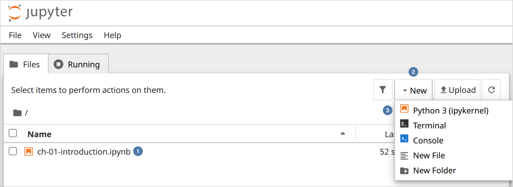
The command is the same on macOS, Linux, and Windows. Jupyter prints a few lines of log in the terminal and opens a browser tab listing the files in the folder you started it from. Keep the terminal open while you work, because closing it stops Jupyter. To open a notebook you have, such as this chapter’s companion notebook, click its name. To make a new one, choose New and then Python 3 (ipykernel) (Figure 1.1): started from webdata, that kernel is that environment’s Python.
A notebook consists of cells. Code cells contain Python that you can execute with Shift+Enter. Markdown cells contain formatted text for documentation. The ability to interleave code with narrative explanation makes notebooks ideal for the kind of exploratory, iterative work that characterizes web data science.
In the companion notebook, this code cell sits under a Markdown cell that holds the paragraph above, as Figure 1.2 shows.
![Screenshot of the notebook ch-01-introduction in Jupyter, with the menus File to Help, Not Trusted at the right, and a toolbar ending in marker 4, the kernel Python 3 (ipykernel). Marker 1: a Markdown cell, the paragraph beginning A notebook consists of cells. Marker 2: a code cell's prompt, [1]:, beside a comment and a print call for Hello, web data science! Marker 3: its output, Hello, web data science!](images/ch-01/jupyter-cells_annotated.png)
[1]: ②, and its output ③ is under it. The kernel, Python 3 (ipykernel), is named at the right of the toolbar ④. Not Trusted, above it, is Jupyter’s label for a notebook you didn’t make on this computer; it doesn’t stop cells from running.
For a thorough introduction to Jupyter Notebooks — cell types, execution order, keyboard shortcuts, kernel management, and common pitfalls — see Missing Manual Chapter 16: Jupyter.
1.3.3 Core Libraries
This book uses several Python libraries extensively, and you installed all of them into webdata along with Jupyter. For now, confirm in a notebook that the ones the first chapters use import without error:
If an import fails with ModuleNotFoundError, the notebook is running a different Python than webdata. Close Jupyter, run conda activate webdata in the terminal, and start jupyter notebook again.
1.4 Your First Request
Let us preview the loop that structures every chapter in this book: retrieve data from the web, parse it into a usable structure, and analyze it to produce insight.
1.4.1 Meet requests
Nearly everything in this book starts with the requests library. It is the standard way to fetch things from the web in Python — its documentation calls it “HTTP for Humans.” When you type a URL, your browser sends a request across the internet, receives a reply, and renders that reply as a page. requests does the same sending and receiving, but instead of rendering the reply, it hands the whole thing to you, as a Python object you can inspect, parse, and analyze.
Why this library and not another? Python ships with a built-in module for the job (urllib), but it is verbose where requests is direct: fetching a page is one readable line, and the library quietly handles the details — character encodings, redirects, connection management — that you should not have to think about in week one. And requests is the ecosystem’s common ground: the scraping and API libraries you will meet later in this book are built on top of it, imitate its interface, or assume you will pair them with it, so the habits you form here transfer everywhere. What actually happens on the wire when a request is sent — protocols, servers, DNS, the anatomy of HTTP itself — is a story worth telling properly, and Chapter 5 tells it. For now, treat requests as a well-made black box: ask for a page, get a reply.
Here you will retrieve the Wikipedia article for the University of Colorado Boulder. Wikipedia refuses requests that don’t say who is sending them, answering requests’ default with a 403, so this one carries a User-Agent header that names you. Put your own email address in it; Chapter 2 explains why sites ask for this.
import requests

# Identify yourself: Wikipedia answers the library's default User-Agent with a 403
headers = {"User-Agent": "WebDataScience/1.0 (your-email@colorado.edu)"}

# Retrieve the page
url = "https://en.wikipedia.org/wiki/University_of_Colorado_Boulder"
response = requests.get(url, headers=headers)

# Check the response
print(response.status_code)  # 200 means success
print(type(response))        # <class 'requests.models.Response'>
print(len(response.text))    # Number of characters in the HTML
That response variable is a Response object — you will handle one every time you touch the web from now on. It is the parcel the server sent back, still in its packaging: not just the page you asked for, but everything about the exchange — whether it succeeded, what kind of document came back, the document itself in two forms, and a record of how you got there. A quick tour of the parts you will actually use:
# What kind of document did the server send?
print(response.headers["Content-Type"])
# text/html; charset=UTF-8

# The body, decoded to text for you -- and the same body as raw bytes
print(type(response.text))     # <class 'str'>
print(type(response.content))  # <class 'bytes'>

# Where you ended up, and how -- redirects leave a trail
print(response.url)      # https://en.wikipedia.org/wiki/University_of_Colorado_Boulder
print(response.history)  # [] -- no redirects this time
The status code you printed above is the server’s three-digit verdict on your request: codes starting with 2 mean success, 4 means something is wrong with your request, and the full taxonomy waits in Chapter 5. The headers are a dictionary of metadata about the reply, and Content-Type is the one you will consult most — it is how you know whether you received HTML to parse, JSON to decode, or something else entirely. The body comes in two forms: .text is the decoded string you will use for web pages, while .content is the raw bytes, which matters when the thing you retrieved is not text at all — a PDF (Chapter 9) or an image has no meaningful .text. And .url with .history tell you where you actually landed: servers routinely redirect requests, and these attributes preserve the trail. One more member of the family, .json(), parses a JSON body into a Python dictionary — this page is HTML so there is nothing for it to parse here, but you will use it within the next few paragraphs.
You can inspect the first 500 characters of the body:
This is raw HTML — not yet useful for analysis. It is the page before a browser draws it, as Figure 1.3 shows side by side. In Chapter 4 and Chapter 6, you will learn to parse this HTML into structured data using BeautifulSoup. For now, the point is that retrieving a web page programmatically is as simple as requests.get(url).
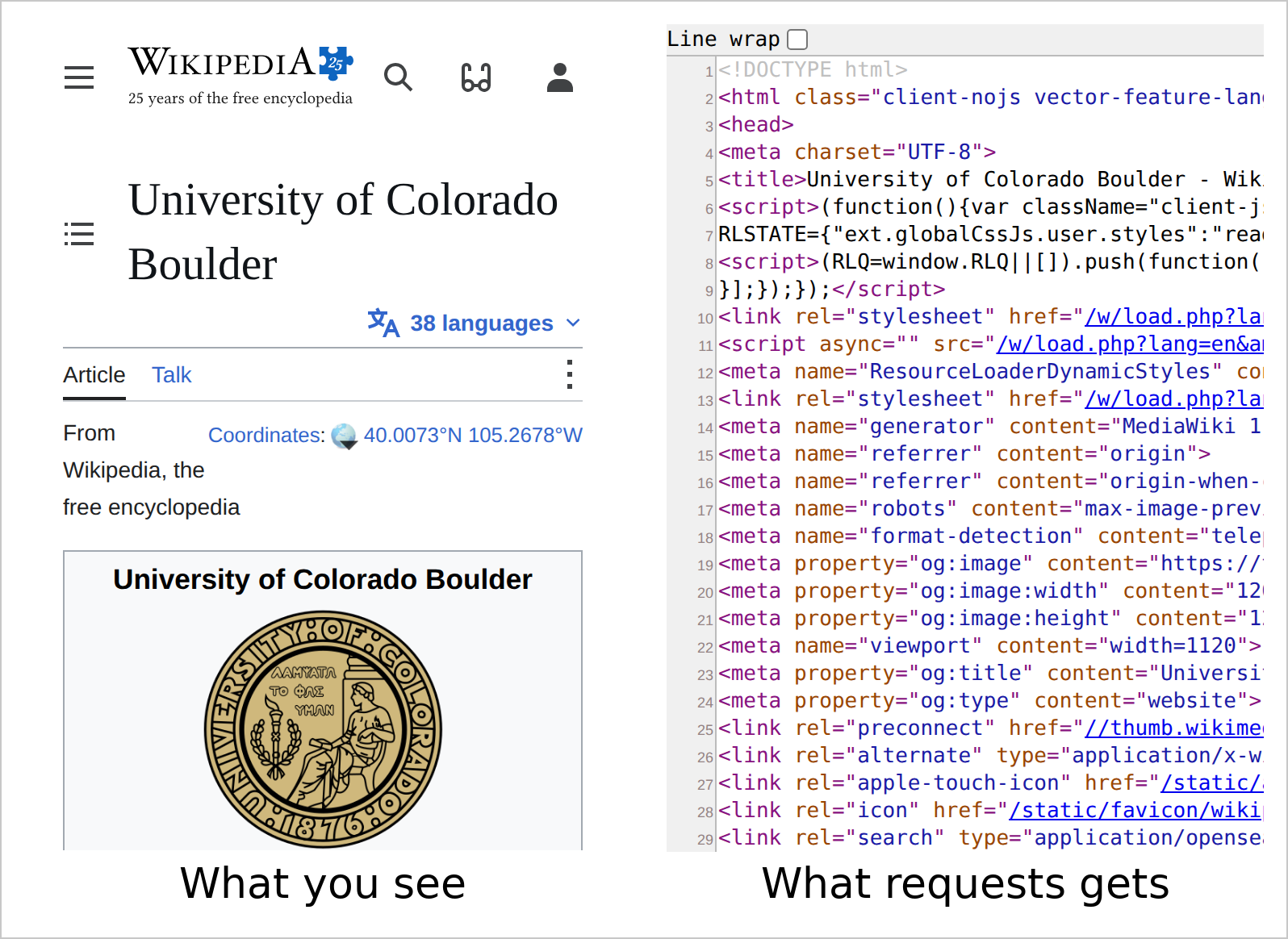
requests.get() returns as response.text. Line 5’s <title> is the heading on the left. The source’s long lines run past the right edge.
1.4.2 Calling Your First API
You can also retrieve data in JSON format from an API. Here is a request to the Wikimedia pageviews API, which returns the number of times a Wikipedia article was viewed on a given day:
import requests

api_url = "https://wikimedia.org/api/rest_v1/metrics/pageviews/per-article"
article = "University_of_Colorado_Boulder"
url = f"{api_url}/en.wikipedia/all-access/all-agents/{article}/daily/20260101/20260131"

headers = {"User-Agent": "WebDataScience/1.0 (your-email@colorado.edu)"}
response = requests.get(url, headers=headers)

data = response.json()  # Parse the JSON response into a Python dictionary
print(type(data))        # <class 'dict'>
print(data.keys())       # What keys are in the response?
Notice two things. First, as with the article, you included a custom User-Agent header identifying yourself and providing contact information. This is a norm of responsible web data collection that you will learn more about in Chapter 2. Second, the .json() method converts the response body from a JSON string into a Python dictionary — a data structure you already know how to navigate. To see that structure before Python has it, paste the same URL into Chrome and tick Pretty-print, as Figure 1.4 shows.
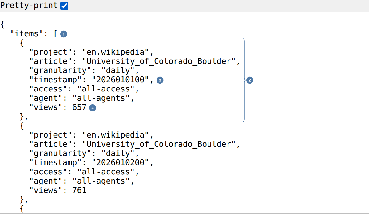
items ①, holds a list with one dictionary per day ②. Each day has a timestamp ③, written year, month, day, and hour, and its views ④: the two fields the plot below is drawn from.
1.4.3 From Response to DataFrame
The data["items"] key contains a list of dictionaries, one per day, each with fields like timestamp, views, article, and project. This is exactly the kind of structure that pandas can convert into a DataFrame with a single call:
import pandas as pd

# Convert the list of dictionaries into a DataFrame
df = pd.DataFrame(data["items"])
print(df.head())
# You'll see columns: project, article, granularity, timestamp, access, agent, views

# The timestamp column looks like "2026010100" — convert it to a proper date
df["date"] = pd.to_datetime(df["timestamp"], format="%Y%m%d00")

# Plot the time series
import matplotlib.pyplot as plt

plt.figure(figsize=(10, 4))
plt.plot(df["date"], df["views"])
plt.xlabel("Date")
plt.ylabel("Daily Pageviews")
plt.title(f"Wikipedia Pageviews: {article}")
plt.xticks(rotation=45)
plt.tight_layout()
plt.show()
This retrieve-parse-DataFrame-visualize pipeline is the fundamental pattern of this book. In every subsequent chapter, you will repeat these steps with different data sources: retrieve HTML pages, XML feeds, JSON API responses, or PDF documents; parse them into structured records; convert those records into a pandas DataFrame; and analyze or visualize the result. The specifics change — BeautifulSoup for HTML, json.loads() for JSON, regular expressions for messy text — but the loop remains the same. Recognizing this pattern early will help you approach each new chapter with a clear mental model of what you are trying to accomplish.
The DataFrame also gives you immediate analytical power. You can compute summary statistics with df["views"].describe(), identify the highest-traffic day with df.loc[df["views"].idxmax()], or resample the data to weekly totals. These operations are not the focus of this chapter, but they illustrate why getting data into a DataFrame is such a valuable intermediate step.
1.4.4 Saving Your Work
Once you have data in a DataFrame, save it to disk — a core practice of responsible web data science:
Serialization — saving your data to a file — matters for three reasons. First, courtesy: every API call consumes server resources, and re-requesting data you already have is wasteful. Second, reproducibility: if you save the data you retrieved on a specific date, your analysis can be reproduced even if the API changes or goes offline. Third, the data itself may change — Wikipedia pageview counts are finalized after a short delay, and an article’s content can be edited at any moment. The version you retrieved is a snapshot, and saving it preserves that snapshot. You will explore JSON serialization for more complex data structures in Chapter 4.
1.5 Documentation as Professional Practice
Your previous classes may have discouraged using online resources. The training wheels are off now. Finding, reading, interpreting, and applying documentation is an essential professional skill, and it is the primary way that working programmers, data scientists, and researchers learn to use new tools.
Bookmark the documentation for the libraries you will use throughout this book:
- requests: requests.readthedocs.io
- BeautifulSoup: crummy.com/software/BeautifulSoup/bs4/doc
- pandas: pandas.pydata.org/docs
- matplotlib: matplotlib.org/stable
When you encounter an error or do not know how to do something, start with the official documentation. If that does not help, search for the specific error message. When asking for help — from a classmate, an instructor, or an AI tool — “it’s not working” is not an actionable request. Describe what you tried, what you expected to happen, what actually happened, and what the error message says.
For strategies on asking effective technical questions and reading official documentation, see Missing Manual Chapter 2: Asking Technical Questions and Chapter 5: Reading Official Documentation.
1.6 Recommended Exercises
This guided exercise is the chapter’s take-home assignment. Work through it in the companion notebook, filling in each empty code cell, and submit the completed notebook. The steps build on one another, so do them in order — everything you need appears in this chapter.
Since this is the first chapter, the assignment is deliberately modest: prove that your environment works, then run the retrieve–parse–analyze loop once, end to end, on an article you choose.
Step 1 — Verify your environment. Import requests, pandas (as pd), and matplotlib.pyplot (as plt). If any import fails, revisit the setup section before going further.
Step 2 — Make your first request. Use requests.get() to retrieve any web page you choose, sending a User-Agent header with your email as the chapter does. Print the status code and the length of response.text.
Step 3 — Call the pageviews API. Pick a Wikipedia article you are curious about. Using the pageviews API URL pattern from this chapter — including the User-Agent header with your email — retrieve its daily views for one full month, and parse the response with .json().
Step 4 — Build a DataFrame. Convert data["items"] into a DataFrame, and convert the timestamp column into a real date with pd.to_datetime(), as the chapter demonstrates.
Step 5 — Plot the time series. Create a line plot of daily views across your month, with labeled axes and a title naming the article.
Step 6 — Save and reload. Save the DataFrame to a CSV file with to_csv(), then load it back with pd.read_csv() and print how many rows you recovered.
Step 7 — Interpret. In three to five sentences: What was the highest-traffic day, and can you connect it to a real-world event? What does the status code from Step 2 mean? And why did Step 6 matter — what can you now do without touching the network again?
1.7 Additional Exercises
These are open-ended extensions — no scaffold, no fixed path. Use them for further practice or deeper exploration.
Exploring the Response object. Use the
dir()function on arequests.Responseobject to list all its attributes and methods. Identify three attributes not discussed in this chapter and use thehelp()function or online documentation to figure out what they do. Write a brief explanation of each in a Markdown cell.POST vs. GET. Read the
requestslibrary documentation and find the method for making a POST request. In a Markdown cell, explain how POST differs from GET and describe a scenario where you would use each. What kind of data does a POST request typically send, and why would an API require it instead of GET?Multi-article comparison. Retrieve daily pageview data for three Wikipedia articles of your choice over the same month. Save each to a separate CSV file using
df.to_csv(). Load all three back withpd.read_csv()and create a single plot with all three time series on the same axes, with a legend identifying each article. Which article had the most variable traffic, and can you hypothesize why?Graduate extension (INFO 5617). Read the computational social science manifesto by Lazer et al. (2009) — a short, field-defining argument about what digital trace data makes possible. Identify three specific claims the authors make about the promise or the perils of studying society through digital traces, such as claims about data access, privacy, or the capacity of academic institutions to compete with industry. For each claim, write a paragraph connecting it to a concrete technique or data source covered in this book’s table of contents, and assess whether the claim has held up in the years since publication. Submit your response as a Jupyter Notebook that uses Markdown cells for the written analysis.
1.9 Common Issues to Debug
jupyter: command not found(or “not recognized” on Windows): Jupyter isn’t installed in the active environment. Runconda activate webdata, thenconda install -c conda-forge notebook, and startjupyter notebookagain.ModuleNotFoundError: A library is not installed in the Python your notebook runs. In a terminal wherewebdatais active (the prompt starts with(webdata)), runconda install -c conda-forge library-name, then restart your Jupyter kernel. If the library is installed and the error remains, Jupyter was started from another environment: runimport sys; print(sys.executable)in the notebook, and check that the path includeswebdata.- A library imports, but a program that came with it can’t be found: Some conda packages also set an environment variable when you activate
webdata, and Jupyter keeps the variables it had when it started. A kernel gets its variables from Jupyter, so restarting the kernel doesn’t help. Close Jupyter, runconda activate webdataagain, and startjupyter notebook. Selenium is the example in this book: after you addseleniumto an older environment, itsUnable to obtain driver for chromehas this cause (Chapter 8). ConnectionError: Your computer cannot reach the server. Check your internet connection; if you are on a university network, try a different network.- Status code 403 (Forbidden): The server rejected your request, often because you did not include a
User-Agentheader; Wikipedia refusesrequests’ default. Send one with your email, as this chapter’s requests do, and see Chapter 2 for more on headers. - Cells running out of order: Jupyter cells can be executed in any order, which leads to stale variables. When in doubt, restart the kernel and run all cells from the top.
1.10 Key Takeaways
The web is a data source unlike any other — massive, messy, and politically contested. Working with it takes the habits of documentation, skepticism, and ethical reflection that distinguish a data scientist from someone who can run a script. Every technique in this book follows the same basic loop: retrieve data from the web, parse it into a usable structure, and analyze it to produce knowledge. You now have your environment set up and have made your first request. The rest of the book builds from here.
1.11 Further Reading
requestslibrary documentation: https://requests.readthedocs.io/- Jupyter Notebook documentation: https://jupyter-notebook.readthedocs.io/
- Wilson et al. (2017) — practical guidance on scientific computing workflows
- Salganik (2018) — Chapter 1: Introduction, for an overview of social research in the digital age
1.8 Social History and Public Interest
Web data science emerged at the intersection of several traditions. Computational social scientists in the 2000s and 2010s recognized that the web was generating behavioral data at unprecedented scale — traces of how people communicate, collaborate, and organize (Lazer et al. 2009). Data journalists discovered that web scraping could hold institutions accountable by making nominally public data actually analyzable. Civic technologists built tools to make government data accessible to citizens.
All three traditions treat data fluency as a form of power that should serve the public interest. As you develop your skills throughout this book, you will encounter recurring questions about who benefits from web data collection, who is harmed by it, and what obligations come with the ability to automate access to information at scale.
Some of the most consequential data science work of the past decade has come from this tradition. ProPublica’s “Machine Bias” investigation in 2016 used scraped court records to reveal racial bias in criminal risk assessment algorithms — a finding that shaped national policy debates about algorithmic fairness. The Markup’s “Citizen Browser” project recruited a panel of real users to study how Facebook’s news feed algorithm distributed political content, producing evidence that would have been impossible to obtain through the platform’s official research tools. These projects combined technical scraping skills with domain expertise and ethical frameworks to produce knowledge that served the public interest.
The intellectual roots of web data science run deeper than any single investigation. The computational social science manifesto by Lazer et al. (2009) articulated a vision of research that works from the “digital traces” left by online behavior — search queries, social media posts, hyperlink structures, editing histories — to answer questions at population scale. These traces are not designed for research; they are byproducts of ordinary activity. The researcher’s task is to transform them into meaningful evidence while respecting the privacy and dignity of the people who generated them. You will meet this tension — between the analytical power of digital trace data and the ethical obligations it creates — in every chapter of this book.
The tools you learn in this book are not neutral. Web data collection can serve openness — making public information practically accessible — or it can enable surveillance and exploitation. The ethical frameworks in Chapter 2 and the public interest framing in Chapter 3 will help you navigate this tension throughout the course.