house_raw = """<?xml version="1.0" encoding="UTF-8"?>
<MemberData publish-date="July 1, 2026">
  <members>
    <member>
      <statedistrict>CO02</statedistrict>
      <member-info>
        <firstname>Joe</firstname>
        <lastname>Neguse</lastname>
        <party>D</party>
        <state postal-code="CO">
          <state-fullname>Colorado</state-fullname>
        </state>
        <district>2nd</district>
      </member-info>
    </member>
    <member>
      <statedistrict>CO03</statedistrict>
      <member-info>
        <firstname>Jeff</firstname>
        <lastname>Hurd</lastname>
        <party>R</party>
        <state postal-code="CO">
          <state-fullname>Colorado</state-fullname>
        </state>
        <district>3rd</district>
      </member-info>
    </member>
  </members>
</MemberData>"""4 Data Formats: XML and JSON
TipLearning Objectives
- Distinguish between XML and JSON as structured data formats and identify when each is typically encountered
- Parse XML documents using BeautifulSoup’s tree navigation methods
- Navigate nested JSON structures using Python’s native lists and dictionaries
- Convert nested data structures into pandas DataFrames for analysis
- Handle common edge cases in structured data parsing
TipCompanion Notebook
Run this chapter’s code as you read: open the companion notebook (see Appendix A for all of them).
4.1 Why Data Formats Matter
Before you can extract data from the web, you need to understand how data is structured on the web. Every web page, every API response, every data feed uses a format that organizes information in a specific way. The two dominant formats you will encounter are XML (Extensible Markup Language) and JSON (JavaScript Object Notation).
XML is the older format, born from the document-centric web of the 1990s. It represents data as a tree of nested tags — a structure you will recognize when you encounter HTML in Chapter 6. HTML and XML are siblings rather than parent and child: both descend from an older markup standard called SGML, and the HTML you find in the wild is not well-formed XML (only the stricter XHTML dialect is). That looseness is precisely why the forgiving HTML parsers you will meet in Chapter 6 exist. The relationship runs deeper than a shared syntax, though: an entire family of formats is built on XML the way XHTML is — MathML for mathematical notation, SVG for vector graphics, RSS and RDF for syndication and metadata — because “define your own tags” turns out to be a useful property for far more than web pages. When you later meet a .svg file or an RSS feed and its structure feels familiar, that is why: you already know how to read it, because you already know how to read XML. JSON is the newer, lighter format that rose with Web 2.0 and the API economy. It maps directly onto Python’s native data structures — lists and dictionaries — making it especially natural to work with programmatically.
This chapter teaches you to parse both formats, building the foundational skills that every subsequent chapter depends on.
4.2 XML and BeautifulSoup
4.2.1 The Tree Structure
XML organizes data as a hierarchy of nested tags. Each tag can contain text, attributes, and child tags. Here is a simplified example of Congressional member data, using the same tag names as the real U.S. House data feed you will retrieve later in this chapter:
This is still just a string. To search and navigate it, you need to parse it into a data structure that understands the tree relationships. That is what BeautifulSoup does.
4.2.2 Parsing with BeautifulSoup
BeautifulSoup’s "xml" parser is not built in — it is provided by the lxml package, which chapter 1’s webdata includes. If you see a bs4.FeatureNotFound error, your environment was made before lxml was on chapter 1’s list: install it with conda install -c conda-forge lxml in a terminal where webdata is active, and restart your kernel.
The power of BeautifulSoup is in its search methods. The .find() method returns the first tag matching your criteria — searching all descendants, no matter how deeply nested. The .find_all() method returns all matching tags as a list:
# Find all member tags
members = soup.find_all("member")
print(len(members))  # 2

# Access text inside a tag
for member in members:
    first = member.find("firstname").text
    last = member.find("lastname").text
    party = member.find("party").text
    print(f"{first} {last} ({party})")
# Joe Neguse (D)
# Jeff Hurd (R)
Notice that member.find("firstname") works even though <firstname> sits inside a nested <member-info> block — .find() searches the entire subtree beneath a tag. Also notice which names you can reach with dot notation. Shortcuts like soup.members.member only work for tag names that are valid Python identifiers; hyphenated names like <member-info> and <state-fullname> break dot notation (Python would read soup.member-info as subtraction), so you must use .find() for them.
XML tags can also carry attributes — key-value pairs inside the opening tag itself. In this schema, the <state> tag stores the two-letter postal code as an attribute and spells out the full state name in a child tag. BeautifulSoup exposes attributes through dictionary-style bracket notation:
# Attributes are accessed with brackets, text with .text
state_tag = soup.find("state")
print(state_tag["postal-code"])               # CO
print(state_tag.find("state-fullname").text)  # Colorado

# The root tag's attribute records when the file was published
print(soup.find("MemberData")["publish-date"])  # July 1, 2026
Text lives between an opening and closing tag and is read with .text; attributes live inside the opening tag and are read with brackets. Real-world XML uses both, and figuring out which one holds the value you need is half the parsing battle.
4.2.3 Extracting and Counting
A common pattern is extracting all values for a particular tag and then analyzing the distribution:
# Count party affiliations
parties = [m.find("party").text for m in soup.find_all("member")]
print(parties)
# ['D', 'R']

# In a real dataset with all 435 members, you could count:
from collections import Counter
party_counts = Counter(parties)
print(party_counts)
# Counter({'D': 1, 'R': 1}) — with full data you'd see actual totals
The .contents method gives you a list of a tag’s direct children, which is useful for exploring unfamiliar XML structures:
4.2.4 Working with Real XML
Let us retrieve and parse actual Congressional member data. The Office of the Clerk of the U.S. House of Representatives publishes a membership roster at clerk.house.gov in XML format. Its structure is what the synthetic example prepared you for: a root <MemberData> tag with a publish-date attribute, containing a <members> tag, containing one <member> per representative, each with the biographical details nested inside <member-info>. The real file adds two blocks we will ignore here: a <title-info> header before <members>, and a <committee-assignments> block in each <member>. You can check that shape before writing any code by opening the file’s address in Chrome, which draws an XML file that has no stylesheet as a tree you can fold (Figure 4.1).
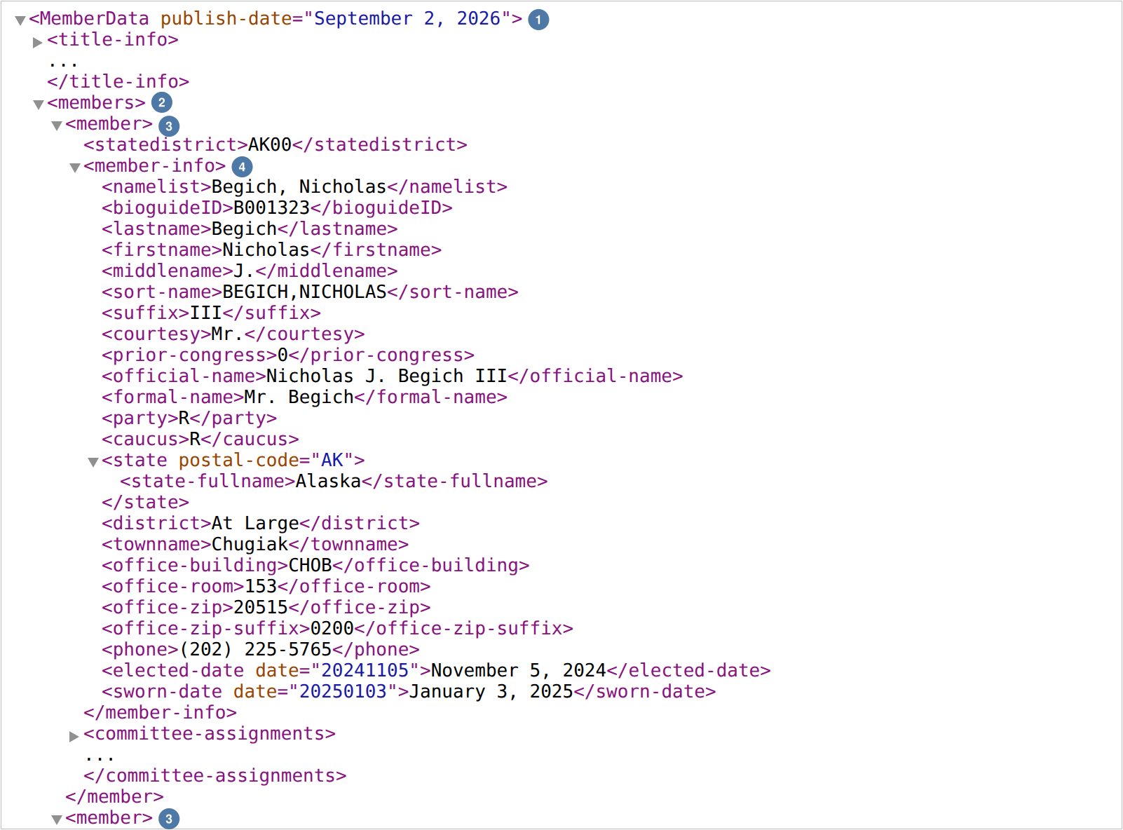
<MemberData> ① with its publish-date, <members> ②, and one <member> ③ per seat, whose biographical details sit in <member-info> ④. The second <member> ③ begins at the bottom. Chrome’s triangles fold <title-info> and the first member’s <committee-assignments>. Chrome’s note above the tree, that the file has no style information, is cropped out.
In Python, fetch the file with requests and parse it with BeautifulSoup’s "xml" parser:
import requests
from bs4 import BeautifulSoup

url = "https://clerk.house.gov/xml/lists/MemberData.xml"
response = requests.get(url)
# Pass the bytes, not response.text: the server names no character set, so .text would guess wrong
soup = BeautifulSoup(response.content, "xml")

# When was this snapshot published?
print(soup.find("MemberData")["publish-date"])
# September 2, 2026

# Find all members
members = soup.find_all("member")
print(f"Total members found: {len(members)}")
# Total members found: 441

# Extract party information
parties = []
for m in members:
    party_tag = m.find("party")
    if party_tag:
        parties.append(party_tag.text)

from collections import Counter
print(Counter(parties))
# Counter({'R': 221, 'D': 217, '': 2, 'I': 1})
Notice response.content rather than response.text. The Clerk’s server labels the file text/xml without naming a character set, so requests falls back to ISO-8859-1, and .text would turn Linda T. Sánchez into “Linda T. Sánchez”. Given the raw bytes, BeautifulSoup reads the encoding the file declares in its first line, UTF-8, and every name comes out right.
Why 441 rather than 435? The file includes the six non-voting delegates and resident commissioner alongside the 435 voting representatives. Your exact counts will also drift as members resign and seats are filled — which is why the publish-date attribute matters. Record it alongside your data so your analysis documents exactly which snapshot of Congress it describes.
That Counter already shows drift in two different ways, and both are worth reading rather than discarding. The two blank-string parties are not a parsing bug: they are vacant seats. The feed’s <member> block for each still exists, but every biographical tag inside it — <firstname>, <lastname>, <party> — is present and empty, and a <footnote> names the reason ("Vacancy due to the resignation of...", with the departing member’s information preserved in a <predecessor-info> block). A seat count of 441 was never a claim that 441 people are serving; it is a claim that 441 lines exist in the roster, two of which are placeholders. And the lone 'I' is Kevin Kiley of California’s 3rd district, whose <party> tag reads I while his <caucus> tag reads R — the schema distinguishes formal party registration from which caucus a member actually sits with, and a Counter over party alone will call him something his colleagues would not. Neither wrinkle shows up unless you go looking; a Counter(parties) that only reports round numbers is one you should not fully trust.
4.2.5 From XML to DataFrame
Counting party affiliations is useful, but the larger payoff is converting the XML into a DataFrame for systematic analysis. The pattern is straightforward: use find_all() to get all records, extract the fields you need from each one, build a list of dictionaries, and pass it to pd.DataFrame():
import pandas as pd

# Extract structured data from each member
records = []
for m in soup.find_all("member"):
    state_tag = m.find("state")  # postal code is an attribute, not text
    record = {
        "first_name": m.find("firstname").text if m.find("firstname") else None,
        "last_name": m.find("lastname").text if m.find("lastname") else None,
        "party": m.find("party").text if m.find("party") else None,
        "state": state_tag["postal-code"] if state_tag else None,
        "district": m.find("district").text if m.find("district") else None,
    }
    records.append(record)

df = pd.DataFrame(records)
print(df.head())
#   first_name last_name party state  district
# 0   Nicholas    Begich     R    AK  At Large
# 1      Barry     Moore     R    AL       1st
# 2    Shomari   Figures     D    AL       2nd
# 3       Mike    Rogers     R    AL       3rd
# 4     Robert  Aderholt     R    AL       4th
Note the state field: because the postal code is stored as an attribute of the <state> tag rather than as its text, we grab the tag once with .find("state") and then use bracket notation — the same pattern you practiced on the synthetic example. The district column contains strings like "1st" and "At Large" rather than numbers, a reminder that XML gives you text and any type conversion is your job.
With the full Congressional dataset, you can now perform real analysis:
# Party breakdown
print(df.groupby("party").size())
#
#     2
# D    217
# I      1
# R    221
# dtype: int64

# Top 10 states by number of representatives
print(df.groupby("state").size().sort_values(ascending=False).head(10))
# state
# CA    52
# TX    38
# FL    28
# NY    26
# IL    17
# PA    17
# OH    15
# GA    14
# NC    14
# MI    13
# dtype: int64
The empty-string party appears here too, sorted before "D" because pandas orders group keys alphabetically and an empty string sorts first. If you wanted only the 439 members actually serving, df[df["party"] != ""] drops the two vacancies before you count.
This find_all → extract fields → list of dictionaries → DataFrame pipeline is the parsing half of the book’s retrieve–parse–analyze loop. You will use it to parse HTML tables in Chapter 6, extract data from archived web pages in Chapter 7, and process PDF text in Chapter 9. The data source changes, the tag names change, but the pipeline stays the same. Once you internalize this pattern, every new parsing challenge becomes a question of “what tags contain the data I need?” rather than “how do I get data into a DataFrame?”
The conditional checks (if m.find("firstname") else None) protect against missing tags — a common issue with real-world XML where not every record contains every field. Without these checks, a single missing tag would crash your entire extraction loop with an AttributeError.
Once the data is in a DataFrame, you have the full power of pandas at your disposal. You can filter members by state (df[df["state"] == "CO"]), compute cross-tabulations of party by state (pd.crosstab(df["state"], df["party"])), or merge Congressional data with external datasets like election results or demographic information. The DataFrame is the universal intermediate format — regardless of whether your data started as XML, JSON, HTML, or PDF text, getting it into a DataFrame is the step that unlocks analysis. This chapter introduces the pattern with XML; the chapters that follow apply it to every other data source on the web.
4.3 JSON and Python Data Structures
4.3.1 Lists and Dictionaries
JSON maps onto two Python data structures you already know. A JSON array is a Python list — ordered, indexed by position:
A JSON object naturally maps to a Python dictionary, which is accessed by key. Python dictionaries preserve insertion order, but JSON object member order should not be relied on:
4.3.2 Nested Structures
Real-world JSON data nests these structures inside each other. A dictionary can contain lists, lists can contain dictionaries, and the nesting can go several levels deep:
The skill of navigating nested structures — working from the outside in, one key or index at a time — is essential for parsing API responses. When you encounter a complex JSON response, start by checking type() and .keys() at the top level, then work your way down.
4.3.3 The List-of-Dictionaries Pattern
The most common JSON pattern you will encounter in web data is a list of dictionaries, where each dictionary represents a record and each key-value pair represents a field:
This pattern converts directly into a pandas DataFrame:
This list-of-dictionaries-to-DataFrame pipeline is the standard way to convert API responses into analyzable data. You will use it in nearly every chapter from here forward.
4.3.4 Parsing JSON Strings
When you receive JSON data from the web (as a string), you need to parse it into Python objects. Python’s built-in json module does the work; its documentation lists every option these functions take:
import json

# Parse a JSON string into a Python object
json_string = '{"name": "Colorado", "population": 5773714}'
data = json.loads(json_string)  # loads = "load string"
print(type(data))    # <class 'dict'>
print(data["name"])  # "Colorado"

# The reverse: convert a Python object to a JSON string
json_output = json.dumps(data, indent=2)  # dumps = "dump string"
print(json_output)
When working with requests, the .json() method on a response object does this parsing for you automatically:
response = requests.get("https://jsonverse.dev/examples/json-metrics.json")
data = response.json()  # Equivalent to json.loads(response.text)
print(data)
# {'metric': 'cpu_usage', 'unit': 'percent', 'interval': '1m',
#  'series': [{'ts': 1698000000, 'value': 45.2}, {'ts': 1698000060, 'value': 48.1}, ...],
#  'tags': {'host': 'server-01', 'region': 'us-east-1'}}
4.3.5 Working with a Real JSON Object
Here is a simplified version of a social media post object, similar to what Twitter’s API used to return:
tweet = {
    "id": 266031293945503744,
    "text": "Four more years.",
    "created_at": "Wed Nov 07 04:49:06 +0000 2012",
    "user": {
        "name": "Barack Obama",
        "screen_name": "BarackObama",
        "followers_count": 23456789
    },
    "entities": {
        "hashtags": [],
        "user_mentions": [],
        "urls": []
    },
    "retweet_count": 814974,
    "favorite_count": 302015
}

# Top-level keys
print(tweet.keys())
# dict_keys(['id', 'text', 'created_at', 'user', 'entities', ...])

# Nested access
print(tweet["user"]["screen_name"])  # "BarackObama"
print(tweet["created_at"])            # "Wed Nov 07 04:49:06 +0000 2012"

# Check for mentions
print(len(tweet["entities"]["user_mentions"]))  # 0
4.3.6 Handling Deeply Nested JSON
The Twitter example above is only two levels deep. Real API responses often nest data three or four levels down, and the path to the data you need is not always obvious. Let us work through a live example using the Open-Meteo weather API, which returns a forecast for Boulder, Colorado:
import requests

url = "https://api.open-meteo.com/v1/forecast"
params = {
    "latitude": 40.01,
    "longitude": -105.27,
    "daily": "temperature_2m_max,temperature_2m_min",
    "timezone": "America/Denver"
}

response = requests.get(url, params=params)
data = response.json()

# Start by understanding the top-level structure
print(type(data))       # <class 'dict'>
print(data.keys())      # dict_keys(['latitude', 'longitude', 'daily', 'daily_units', ...])

# The daily data is nested one level down
print(type(data["daily"]))      # <class 'dict'>
print(data["daily"].keys())     # dict_keys(['time', 'temperature_2m_max', 'temperature_2m_min'])

# The actual values are lists inside the 'daily' dictionary
print(data["daily"]["time"][:3])              # ['2026-09-09', '2026-09-10', '2026-09-11']
print(data["daily"]["temperature_2m_max"][:3]) # [28.4, 31.2, 32.6]

# Use .get() for safe access with a default
elevation = data.get("elevation", "unknown")
print(f"Elevation: {elevation} meters")
# Elevation: 1635.0 meters
The address in url is only half of the request. Opened on its own in a browser, https://api.open-meteo.com/v1/forecast returns an empty page, because the parameters are what ask for a forecast. requests adds them to the address for you, and print(response.url) shows the full URL it sent, which you can paste into a browser to see the same JSON (Figure 4.2).
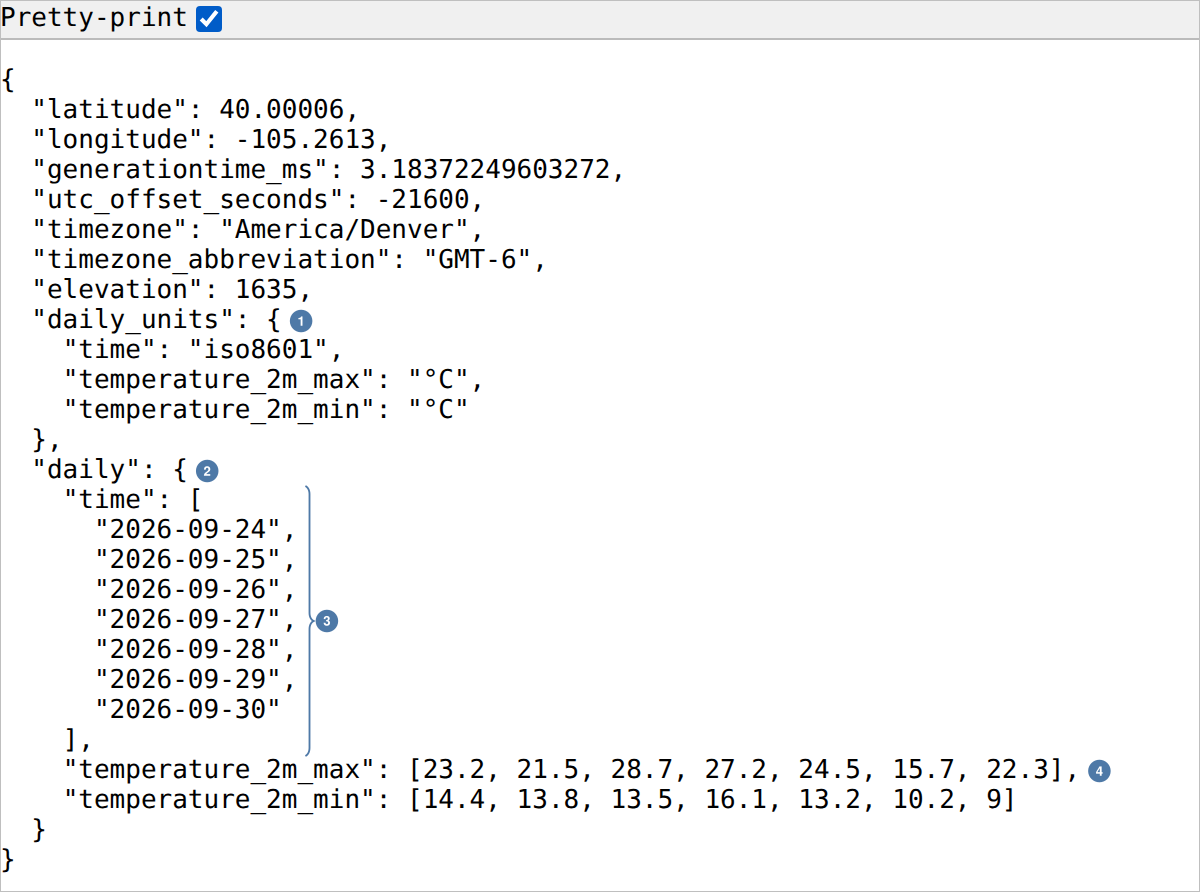
daily_units ① gives each list’s unit, and daily ② holds the data. Its time ③ and temperature_2m_max ④ are parallel lists, one entry for each of seven days, so data["daily"]["temperature_2m_max"][0] is the first day’s high. Pretty-print drops a whole number’s .0 (1635), which Python keeps (1635.0).
The strategy is always the same: start with type() and .keys() at the top level, then work inward one key at a time. When you find the lists you need, convert them to a DataFrame:
import pandas as pd
import matplotlib.pyplot as plt

df = pd.DataFrame({
    "date": pd.to_datetime(data["daily"]["time"]),
    "high": data["daily"]["temperature_2m_max"],
    "low": data["daily"]["temperature_2m_min"],
})

plt.figure(figsize=(10, 4))
plt.plot(df["date"], df["high"], label="High", color="red")
plt.plot(df["date"], df["low"], label="Low", color="blue")
plt.fill_between(df["date"], df["low"], df["high"], alpha=0.2)
plt.xlabel("Date")
plt.ylabel("Temperature (°C)")
plt.title("Boulder, CO — 7-Day Forecast")
plt.legend()
plt.tight_layout()
plt.show()
The .get() method is your most important tool for navigating unfamiliar JSON. Unlike bracket notation (data["key"]), which raises a KeyError if the key is missing, .get("key", default) returns the default value silently. This is especially useful when API responses vary — some records might include optional fields that others omit.
Notice the general strategy for tackling any unfamiliar JSON response. First, check the type and keys at the top level. Then pick the key that looks most relevant and repeat the process one level deeper. Continue until you find the lists of values you need. This “peel the onion” approach works regardless of how deeply nested the data is, and it avoids the common mistake of trying to write complex extraction code before you understand the structure. You will use this strategy repeatedly in Chapter 10, Chapter 11, and Chapter 12 when working with APIs that return richly structured JSON responses.
4.4 When to Use Which
Neither format is simply better than the other — each makes different trade-offs, and those trade-offs are exactly why each one turns up where it does. The comparison holds regardless of which library does your parsing:
| XML | JSON | |
|---|---|---|
| Size and readability | Verbose: every element needs a matching closing tag | Compact: braces and brackets, no repeated tag names |
| Native language support | Needs a parser library in every language, JavaScript included | Parses natively in JavaScript (JSON.parse); near-universal library support elsewhere |
| Structural vocabulary | Rich: elements, attributes, mixed text-and-markup content, namespaces for combining vocabularies | Simple: objects, arrays, strings, numbers, booleans, null |
| Schema and validation | Mature: DTD and XML Schema (XSD) let you enforce a document’s shape before anything tries to parse it | Looser: JSON Schema exists but is newer and less universally adopted |
| Display capability | Can double as a document format — the markup itself can carry rendering instructions, which is what XHTML, SVG, and Office file formats rely on | Purely a data format; no display semantics at all |
| Comments | Allowed | Not allowed — a real documentation gap every JSON author eventually hits |
| Typing | Everything parses as text; converting "223" to an integer is your job, as you saw above |
Preserves numbers and booleans through parsing without extra conversion |
4.4.1 Where you’ll actually find each format
Format choice is rarely arbitrary once you know what to look for. JSON dominates anywhere a program is the primary reader. REST APIs return it almost by default now — SOAP, the XML-based protocol REST displaced, requires wrapping every request in an XML namespace envelope that JSON has no equivalent for, which is part of why SOAP’s use has been declining for years while REST and GraphQL have grown. JSON Web Tokens (JWTs), the credential your browser holds after you log into a site, are JSON underneath. Configuration files for modern developer tooling — package.json, tsconfig.json, VS Code’s settings.json — are JSON because the ecosystem around them is JavaScript-adjacent and a program on both ends is doing the reading.
XML persists where a human sometimes needs to read the document, where a strict contract matters, or where the data predates the JSON era. Government and legislative systems (the House roster you are about to parse), SEC filings, and enterprise data-interchange formats still commonly use XML, partly out of legacy and partly because XSD validation gives an institution a way to guarantee — mechanically, not by convention — that a submitted document has the fields it is supposed to have. RSS and Atom feeds are XML for historical reasons this chapter’s next section covers. And XML shows up somewhere many people never notice: open a .docx, .xlsx, or .svg file’s internals, and you are looking at XML. Office Open XML files are literally a zip archive of XML documents; SVG is XML that a browser renders directly as a vector image. Wherever a format needs to be both a document and data at once, XML’s willingness to carry markup alongside content is doing real work that JSON, by design, cannot.
HTML — which you will parse extensively beginning in Chapter 6 — is structurally similar to XML and is parsed with the same BeautifulSoup methods.
NotePublic Interest Connection
The choice of data format is itself a transparency decision. When governments and institutions publish data in machine-readable XML or JSON, they embody openness — making information practically accessible to anyone with basic programming skills. When the same data is published as scanned PDFs or proprietary spreadsheets, it creates barriers to the kind of oversight that democratic accountability requires (Chapter 3). Advocating for open data formats is one of the most concrete things a data scientist can do to serve the public interest.
TipMissing Manual Reference
For more on data file formats including CSV, TSV, and other common structures, see Missing Manual Chapter 20: Data File Formats.
4.5 Recommended Exercises
This guided exercise is the chapter’s take-home assignment. Work through it in the companion notebook, filling in each empty code cell, and submit the completed notebook. The steps build on one another, so do them in order — everything you need appears in this chapter or an earlier one.
You will parse one real dataset in each format: an RSS feed (XML) and a weather forecast (JSON), ending with both as DataFrames.
Step 1 — Set up politely. Define your HEADERS with a named User-Agent (Chapter 2). Find an RSS feed from a news outlet or podcast — most sites serve one at /rss or /feed — and check the site’s robots.txt permits fetching it.
TipStarter feeds
Five news outlets and five data/tech podcasts, researched as of September 2026. RSS URLs move over time — treat these as a starting point, not a guarantee; the status-code check in Step 2 is exactly how you’d notice if one has moved.
News
| Outlet | Feed |
|---|---|
| The New York Times | https://rss.nytimes.com/services/xml/rss/nyt/HomePage.xml |
| BBC News | https://feeds.bbci.co.uk/news/rss.xml |
| The Guardian | https://www.theguardian.com/world/rss |
| PBS NewsHour | https://www.pbs.org/newshour/feeds/rss/headlines |
| Al Jazeera | https://www.aljazeera.com/xml/rss/all.xml |
AP and Reuters are conspicuously absent: both discontinued their public RSS feeds (Reuters in 2020, AP some time after) — a small, real instance of the decline this chapter describes below.
Podcasts (data, tech, and data journalism)
| Podcast | Feed |
|---|---|
| Data Skeptic | https://dataskeptic.libsyn.com/rss |
| Planet Money (NPR) | https://feeds.npr.org/510289/podcast.xml |
| The Changelog | https://changelog.com/podcast/feed — note: its robots.txt disallows all crawlers, so this feed fails Step 1’s check |
| Data Engineering Podcast | no single published URL — find it on dataengineeringpodcast.com using the technique below |
| The PolicyViz Podcast | no single published URL — find it on policyviz.com/podcast using the technique below |
Finding a feed this list doesn’t cover. Most sites don’t advertise their feed on the homepage:
- Try appending
/rss,/feed, or/rss.xmlto the site’s root URL — the most common convention. - View the page source, not the rendered page (right-click the page and choose View Page Source, or press Ctrl + U; ⌘ + ⌥ + U on a Mac), and search it for
application/rss+xml. The<link>tag with thattypenames the feed’s address in itshref, even when nothing on the page itself links to the feed (Figure 4.3). - For a podcast specifically, check its listing on a podcast directory (Apple Podcasts, Podchaser, Listen Notes) — most display or link to the canonical feed even when the show’s own site doesn’t.
- Look for a small RSS icon or a “Subscribe” link, often in a page footer or sidebar.

application/rss+xml, September 2026. The one match is on line 33, in a <link rel="alternate"> whose href ① is the feed’s address. The address bar shows the view-source: prefix; typed before any address, it opens that page’s source.
Step 2 — Fetch and inspect the XML. Retrieve the feed with requests. Print the status code and the first 500 characters. Identify the repeating element by eye — for RSS it is <item>. Chrome draws a feed served as XML as a tree you can fold (Figure 4.4), and a feed served as application/rss+xml, such as PBS NewsHour’s, as plain text.
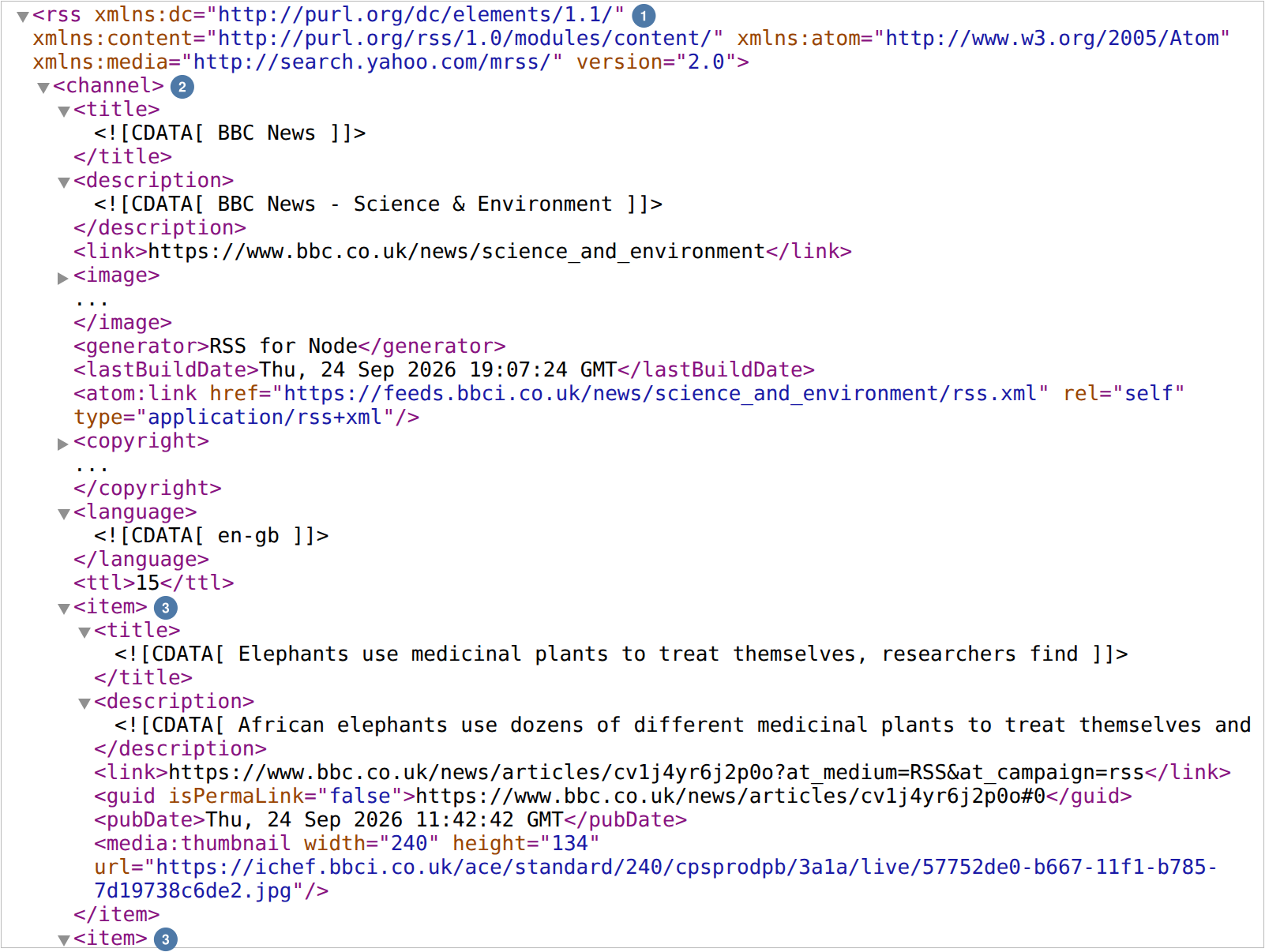
<rss> ① holds one <channel> ②: the feed’s title, description, and link, then one <item> ③ per story, each with a title, description, link, guid, date, and thumbnail; the second <item> ③ begins at the bottom. Each CDATA wrapper marks text the parser takes as it is, and BeautifulSoup’s .text returns what is inside. The channel’s <image> and <copyright> are folded, and Chrome doesn’t wrap CDATA, so the first description runs past the edge.
Step 3 — Parse the tree. Parse the response with BeautifulSoup’s "xml" parser, use find_all() to collect the items, and print how many the feed contains.
Step 4 — Extract to a DataFrame. Loop over the items, building a list of dictionaries with each item’s title, link, and publication date — the list-of-dictionaries pattern from this chapter — then convert to a DataFrame.
Step 5 — Fetch nested JSON. Retrieve the Boulder forecast from https://api.open-meteo.com/v1/forecast?latitude=40.01&longitude=-105.27&daily=temperature_2m_max&timezone=America/Denver and parse it with .json(). Print the top-level keys, then the keys under "daily" — map the nesting before you extract anything.
Step 6 — Extract the parallel lists. The "daily" object holds parallel lists of dates and temperatures. Build a DataFrame from them and plot maximum temperature over the forecast days.
Step 7 — Interpret. In three to five sentences: The RSS feed nested repeating elements; the forecast nested parallel lists. Which was easier to get into a DataFrame, and why? What did you have to know about each structure before you could write the extraction code?
4.6 Additional Exercises
These are open-ended extensions — no scaffold, no fixed path. Use them for further practice or deeper exploration.
XML vs. JSON comparison. Find a data source that provides the same information in both XML and JSON formats (e.g., a government API or data service). Retrieve both versions and compare: how does the structure differ? Which is easier to parse in Python? Which contains more metadata?
Reusable extraction function. Write a function
xml_to_dataframe(soup, tag_name, fields)that takes a BeautifulSoup object, the name of the repeating tag (e.g.,"member"), and a list of child tag names to extract (e.g.,["firstname", "lastname", "party"]). The function should return a DataFrame. Test it on the Congressional XML from this chapter, then try it on an RSS feed (where the repeating tag is"item"and the fields might be["title", "link", "pubDate"]).Weather data analysis. Retrieve a 7-day forecast from the Open-Meteo API for Boulder, CO using the URL pattern from this chapter. Navigate the nested JSON response, build a DataFrame with dates and both high and low temperatures, and create a plot showing both temperature series. Add a horizontal line at 0°C and annotate any days where the low drops below freezing.
Graduate extension (INFO 5617). Select a public XML or JSON dataset in the wild — a data.gov feed, an SEC EDGAR filing, a city open-data API, or something from your own research area. Write a datasheet-style critique of it in the spirit of Gebru et al. (2021): what does the schema and its documentation tell you (or fail to tell you) about how the data was collected, what its fields mean, and what uses it was designed for? Evaluate concrete design choices — attributes versus child tags, nesting depth, naming conventions, the presence or absence of a published schema — and how each helps or hinders a researcher trying to reuse the data. Conclude with two specific recommendations the publisher could adopt to improve interoperability and documentation.
4.8 Common Issues to Debug
- Parser selection: Use
"xml"for XML documents and"html.parser"or"lxml"for HTML. Using the wrong parser produces unexpected results. json.JSONDecodeError: The string is not valid JSON. Common causes include trailing commas, single quotes (JSON requires double quotes), or the response containing HTML error pages instead of JSON.KeyErrorin dictionaries: The key does not exist. Use.get("key", default_value)for safe access.- Garbled accented letters, such as
SánchezforSánchez:requestsdecoded the body with the wrong character set, usually because the server’sContent-Typeheader names none;requeststhen falls back to ISO-8859-1. Passresponse.contentto BeautifulSoup so the parser reads the encoding the document declares, or setresponse.encoding = "utf-8"before readingresponse.text. - Confusion between
json.loads()andjson.load():loadsparses a string;loadparses a file object.
4.9 Key Takeaways
XML and JSON are the two structural languages of web data. XML organizes data as a tree of nested tags; BeautifulSoup makes that tree navigable through .find(), .find_all(), and .text. JSON organizes data as nested lists and dictionaries; Python’s native data structures map directly onto it. The skill of converting nested structures into flat DataFrames — the list-of-dictionaries-to-DataFrame pipeline — is the bridge between raw web data and analysis, and you will use it in nearly every subsequent chapter.
4.10 Further Reading
- BeautifulSoup documentation: https://www.crummy.com/software/BeautifulSoup/bs4/doc/
- Python
jsonmodule: https://docs.python.org/3/library/json.html - W3C XML specification: https://www.w3.org/XML/
- JSON specification: https://www.json.org/
- awesome-rsshub-routes, a health-checked directory of official and RSSHub-generated feeds: https://github.com/JackyST0/awesome-rsshub-routes
- awesome-rss-feeds, a curated list of RSS feeds and OPML files: https://github.com/plenaryapp/awesome-rss-feeds
- RSS.com’s roundup of popular podcast RSS feeds: https://rss.com/blog/popular-rss-feeds/#the-most-popular-podcast-rss-feeds
- Examples of JSON versus XML: https://www.json.org/example.html
- Mitchell (2018) — Chapter 1: Your First Web Scraper
Gebru, Timnit, Jamie Morgenstern, Brenda Vecchione, et al. 2021. “Datasheets for Datasets.” Communications of the ACM 64 (12): 86–92. https://doi.org/10.1145/3458723.
Mitchell, Ryan. 2018. Web Scraping with Python: Collecting More Data from the Modern Web. 2nd ed. O’Reilly Media.
4.7 Social History and Public Interest
XML emerged in the late 1990s from the standardization efforts of the World Wide Web Consortium (W3C), designed to be a universal format for document and data exchange. Its verbosity made it rigorous but heavy. JSON was created by Douglas Crockford in the early 2000s as a lightweight alternative that leveraged JavaScript’s native object syntax. Its simplicity and the rise of AJAX-powered web applications made it the default format for APIs by the 2010s.
The politics of data formats may seem esoteric, but format choices have real consequences for access and transparency. When a government publishes budget data as XML, it is machine-readable by design. When it publishes the same data as a scanned PDF, it is technically “public” but practically inaccessible — a form of the soft enclosure discussed in Chapter 3. Open government data initiatives like data.gov have pushed for machine-readable formats precisely because format determines who can actually use the data.
RSS (Really Simple Syndication) deserves special mention as an early experiment in open data distribution. Built on XML, RSS feeds allowed anyone to subscribe to updates from blogs, news sites, and podcasts without visiting each site individually. In the mid-2000s, RSS was the backbone of the blogosphere and an early tool for computational journalism — researchers could subscribe to thousands of news feeds and analyze coverage patterns at scale. But RSS declined as social media platforms offered their own proprietary feed algorithms. Facebook, Twitter, and later platforms replaced the open, user-controlled subscription model with opaque algorithmic curation. The decline of RSS was one of the earliest examples of the enclosure pattern that Chapter 3 describes: an open protocol replaced by a proprietary system that centralized control over information distribution.